Prediction of Pollutant Removal in the Treatment Plant of Industrial Shahid Salimi Town Using ANN
Vahid Pakrou1 * , Saeed Pakrou1 , Naser Mehrdadi2 and Mohammad Javad Amiri2
1
Civil Engineering – Environmental,
Aras International Campus,
Iran
2
Civil Engineering – Environmental,
University of Tehran,
Iran
http://dx.doi.org/10.12944/CWE.10.Special-Issue1.109
Predicting the pollutant removal of the treatment plant of Shahid Salimi industrial town is performed in this study using artificial neural network. The required data of this treatment plant are achieved by 162 records after eliminating the repeated and uncompleted data. The appropriate inputs (BOD, COD, and TSS) are chosen by the correlation analysis in terms of having the highest correlation with the output parameters of the treatment plant, considering the small size of data sets and the need to simplify the model. The architecture of the network is used to make the proper prediction, which uses one neural network to predict all the output parameters (BOD, COD, and TSS). This network with 20 neurons in two hidden layers could predict the output of the treatment plant with good accuracy. Excellent results indicating the success of the modeling are obtained using the mentioned architecture.
Copy the following to cite this article:
Pakrou V, Pakrou S, Mehrdadi N, Amiri M. J. Prediction of Pollutant Removal in the Treatment Plant of Industrial Shahid Salimi Town Using ANN. Special Issue of Curr World Environ 2015;10(Special Issue May 2015). DOI:http://dx.doi.org/10.12944/CWE.10.Special-Issue1.109
Copy the following to cite this URL:
Pakrou V, Pakrou S, Mehrdadi N, Amiri M. J. Prediction of Pollutant Removal in the Treatment Plant of Industrial Shahid Salimi Town Using ANN. Special Issue of Curr World Environ 2015;10(Special Issue May 2015). Available from: http://cwejournal.org?p=697/
Download article (pdf)
Citation Manager
Publish History
Introduction
Industrial development has direct relation with industry and technology at one hand and destruction and pollution on the other hand. Management of dangerous wastes has become one of the most serious problems of the world today with the emergence of industrial societies and the increasing reliance of human societies on industry and industrial processes, and therefore, pollution analysis and reducing its destructive effects to a reasonable extent and toward sustainable development is urgent to ensure the health in the growth and present and future development of the creatures of the earth (Mahnaz Pashazadeh, 2010). The sullage of industrial units is one of these problems (Chalkesh Amiri, 2010). Malfunctioning of a sewage treatment plant may cause serious problems to the environment and public health (Alireza Mehdipour Torghabeh, 2012). Therefore, the performance of an industrial sewage treatment plant is basically related to local experiences of the procedure engineer, who specifies a special location of the treatment plant (Mohammad Shokuhiyan, 2012). The more complete treatment of industrial sullages becomes more important, for the improper disposal of industrial waste has adverse effects on the environment (Khosravi et al., 2013). Industrial sullages would deplete surface and underground waters in the case of disposal in the environment due to the presence of organic materials and minerals (Metcalf, 2003); in this regard, the optimization and improvement of the current situation of treatment plants got an important position in the field of environment. This is where every improvement needs to be evaluated in the current situation and new situations (Khosravi et al., 2013). However, the prediction of efficiency and performance of the system is not possible by the normal methods because of the complexities in the industrial units. Thus, using artificial intelligence methods such as fuzzy logic and artificial neural networks could simplify this evaluation (Dogan, 2008) and even make the prediction of the system’s performance possible (Guclu & Dursun, 2010). Artificial Neural Networks (ANNs) have been under special consideration in recent years as one of the modern methods in modeling. ANNs could be utilized in modeling the treatment plant processes because of their accuracy and perfect applications and flawless engineering. Therefore, the present study tries to predict the pollutant removal amount of the sullage treatment plant at the Shahid Salimi industrial town using ANNs.
Methods and Materials
An artificial neural network is an idea to process the information, which has been inspired by biological nervous system and processes the information just like the brain. The key element of this idea is the new structure of information processing system. This system consists of a large number of ultra-compact processing elements, which are acting coordinate with each other to solve a problem.
Neural networks, with significant ability to derive meaning from complicated or imprecise data, could be employed in extracting patterns and identifying methods, which are very complex or difficult for human or other computer based techniques to understand. A trained neural network can be considered as a specialist in the information concept that is introduced to be analyzed.
Advantages of Neural Networks
Adaptable learning: the ability to learn the way of doing the tasks based on the information introduced as a training or preliminary experiences.
Self-organization: an artificial neural network can create its organization or presentation of the information it had received during the training stage.
Real time: the calculations of artificial neural network could be performed parallel and special hardware has been designed to use this ability.
Fault tolerance without interruption while coding the information: partial damage leads to degradation of its performance, however, some abilities of the network may remain even with a giant damage.
Learningtypes For Neural Networks
Supervised Learning – Escalation Learning – Learning without Supervisor
Architecture Of Neural Networks
Single-Layer Neywork
Two or more neurons in a layer could combine with each other. A network could be established of one or more layers like this.
Multi-Layer Network
Two or more neurons could combine with each other within a layer. A special network could consist of many layers. Each layer in the network has its own weight matrix, bias vector, and output. This kind of network has vast application in the form of two layers at the back propagation error networks.
Levenberg-Marquardt Training Algorithm
The Levenberg-Marquardt training algorithm benefits from high-speed convergence, because it doesn’t need to solve the Hessian matrix and approximates it by the Jacobian matrix instead. It should be noted that, some problems may occur at calculations when the size of the Jacobian matrix is large, of course there are methods by which there is no need to calculate all the elements of the Jacobian matrix. This algorithm is used here because of its learning capability and high efficiency (Russell and Norvig, 2003). The accuracy of prediction is usually evaluated by providing data which the network is not faced with before, which is known as the network’s ability at Root Mean Square Error (RMSE), Generalization (R). For this purpose, the criteria of correlation coefficient are used to evaluate the designed network Mean Absolute Percentage Error (MAPE) and Mean Absolute Error (MAE).
In which, n is the number of predictions; Yact is the real observed value; real observed value; Yest is the predicted value; Ȳact is the average of real observed value; and Ȳest is the average of predicted value extracted from the model (Mehdipour and Shokouhiyan, 2012).
Results
The received data from the Shahid Salimi treatment plant located at the Shahid Salimi industrial town of Tabriz is used as a black box model for the training of a neural network and modeling the treatment process. The statistical analysis of the data will be explained in the first section. Then the data preparations to be used in the neural network toolbox of the MATLAB software will be discussed. This preparation includes choosing the proper inputs and preprocessing of the inputs and outputs of the network. The results of modeling and its accuracy will be proposed in the next section.
Statistical Analysis
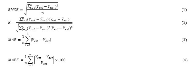
The data used in this research are equal to 162 measured data during the years of 2012 and 2013 from the Shahid Salimi treatment plant laboratory located at the Shahid Salimi industrial town of Tabriz. The graphs of measured variables in the input and output of the treatment plant are shown in figure (1).
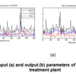 |
Figure 1: Input (a) and output (b) parameters of the Shahid Salimi treatment plant Click here to View figure |
In order to choose the proper inputs for training the neural network so that the complexity of the model becomes as low as possible and simultaneously the accuracy of prediction become maximum, it is necessary to analyze the available data. The complexity of model needs to come down as much as possible with regard to the low number of recorded input and output data, because there are not enough examples to discover the complex relations between all the inputs and outputs. Therefore, it is necessary to choose the best parameters of identifying the model using the correlation analysis between the input and output parameters.
Correlation Analysis
The correlation coefficient is a statistical tool for determining the type and degree of relation between one quantitative variable and another. The correlation coefficient is one of the criteria used in determining the correlation between two variables. The correlation coefficient shows the intensity of a relation and also the type of relation (direct or reverse). This coefficient is between 1 and -1, and is equal to zero in the case of no relation between two variables. The correlation between two random variables X and Y is defined as follows:

In which, E is the expected value operator, cov means covariance, and, corr a widely used alternative notation for the correlation coefficient. The resulting value from the above equation would be 1 by placing Corr (X, X), and -1 by placing Corr (X, -X). As it can be seen, the maximum correlation is 1 at the (X, X) and it obtains a value between 0 and 1 for less correlated variables. This equation is true in the case of having inverse correlation by adding a negative sign to it.
The results of performing the correlation analysis on the input and output data showed that the maximum correlation is between the output parameters of BOD, COD, and TSS and the input parameters of BOD, COD, and TSS. In other words, knowing only these parameters in the input of the treatment plant is enough for the prediction of the output parameters including BOD, COD, and TSS.
Box Plot
The box plot could be used a lot in analyzing the input and output of a system which we want to model it. The box plot for the used inputs in the modeling of the treatment process is shown in the figure (2), which includes BOD, COD, and TSS.
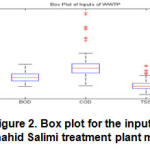 |
Figure 2: Box plot for the inputs of Shahid Salimi treatment plant model Click here to View figure |
Figure (3) shows the box plot for the outputs of the treatment plant model. It can be inferred from the figure that the average of output data is much less than the input, which is accordant with the technical specifications of a treatment plant. On the other hand, the data dispersion in the output is much more than the input. This could be observed from the external boundaries of the box plot, especially for COD.
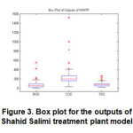 |
Figure 3: Box plot for the outputs of Shahid Salimi treatment plant model Click here to View figure |
Data Preprocessing
Processing at the procedure of updating the weight is done to assign the equal variable weight, especially while using the nonlinear transfer function, according to the distribution of used data in the neural network and after preparing the data to develop the model. Preprocessing of the data is done by allocating the input and output data to the range [0, 1] or [-1, 1]. This transformation is as follows for all the data points:
For the interval [0, 1]:

Each data variable should be fed into the neural network model using normalization of input data with nonlinear transfer functions such as logsig, tansig and with equal weight. Therefore, the data should be scaled by the equations (6) and (7) in the intervals [0, 1] and [-1, 1], respectively.
Model Development
The laboratory data recorded in the treatment plant of Shahid Rajayi industrial town is used for modeling the input and output of the treatment plant. The total of 162 records of inputs and outputs is extracted after removing the incomplete and duplicate data. This amount of data is divided randomly into three sets. Transposing the inputs of neural network does not matter, since the modeling is static and the used neural network (feed forward neural network) is only able to do the static mappings. Therefore, dividing the data set randomly into three groups of training, validation and test is proper. The existing data in the training set are used to train the network. 60 percent of data are used in training, 20 percent in validation and 20 percent in the test of the neural network.
The below architectural approach is considered for the neural network model development, in which the inputs are BOD, COD, and TSS of the Shahid Salimi treatment plant.
Network Architecture
The prediction of all the output parameters in the above architecture is being done by one neural network. This neural network takes the inputs of BOD, COD, and TSS from the treatment plant and predicts the outputs of BOD, COD, and TSS. For this purpose, a feed forward neural network is created in the MATLAB software and in its toolbox by the Levenberg-Marquardt training algorithm and existing data. Initially, this neural network is trained by 10 neurons at two hidden layers. The results of regression analysis for the separate outputs are presented in figure (4).
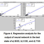 |
Figure 4: Regression analysis for the output of neural network in the test state of a) BOD, b) COD, and d) TSS Click here to View figure |
The results of comparison between different outputs and the real values for BOD, COD, and TSS are presented in figures (5), (6), and (7), respectively. The prediction of BOD and COD has high accuracy, but the comparison of real data and predicted outputs for TSS indicates the average accuracy of the neural network.
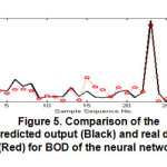 |
Figure 5: Comparison of the predicted output (Black) and real data (Red) for BOD of the neural network Click here to View figure |
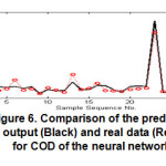 |
Figure 6: Comparison of the predicted output (Black) and real data (Red) for COD of the neural network Click here to View figure |
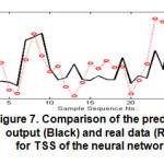 |
Figure 7: Comparison of the predicted output (Black) and real data (Red) for TSS of the neural network Click here to View figure |
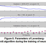 |
Figure 8: Parameters of Levenberg-Marquardt algorithm during the training of neural network Click here to View figure |
The results are better for 20 neurons in each layer. Regression analysis of the test stage is performed for the outputs of the neural network, which is shown in the below figure. The value of R for TSS has improved in comparison to the neural network with 10 neurons in two hidden layers.
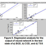 |
Figure 9: Regression analysis for the output of neural network in the test state of a) BOD, b) COD, and d) TSS Click here to View figure |
The results of comparison between different outputs and the real values of BOD, COD, and TSS are shown in the figures (10), (11), and (12). The prediction of BOD and COD is very accurate and has become more accurate compared to the neural network with neuron.
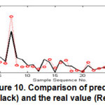 |
Figure 10: Comparison of predicted output (Black) and the real value (Red) for BOD Click here to View figure |
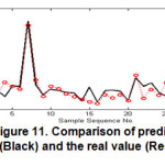 |
Figure 11: Comparison of predicted output (Black) and the real value (Red) for COD Click here to View figure |
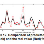 |
Figure 12: Comparison of predicted output (Black) and the real value (Red) for TSS Click here to View figure |
Discussion and Conclusion
A model is developed in this study by the feed forward neural networks and Levenberg-Marquardt training algorithm to predict the outputs of the treatment plant in Shahid Salimi industrial town of Tabriz. The main challenge is the lack of data for training the neural network. Thus, statistical correlation analysis is employed in this research in order to choose proper inputs among the input candidates. Three inputs, including BOD, COD, and TSS were chosen among BOD, COD, TSS, temperature, pH, and dissolved oxygen in aerobic process. These three inputs are the only ones having a significant correlation with the outputs of the treatment plant.
A neural network with three inputs and three outputs were used in the architecture of this research in order to predict the output parameters of the treatment plant (BOD, COD, and TSS), which shows the efficiency of the treatment plant in removing pollutants. This network with 20 neurons in two hidden layers has predicted the outputs of the treatment plant with a very good accuracy. This architecture is sensitive to the number of neurons in hidden layers, and the neural network in this research with 10 neurons in two hidden layers was not able to predict the output TSS with an expected accuracy.
References
- Arsi Vala, , Wastewater Treatment, Translate by Ahmadreza Yazdanbkhsh, Kazem nadafi, Fardabeh Press. (1993)
- Chalkesh Amiri, M., , Principles of water treatment, Esfahan, Arkan Press. (2010)
- Dogan, E. e. a. "Application of Artificial Neural Networks to Estimate Wastewater Treatment Plant," Environmental Progress, 27, (4), 439-445, (2008).
- Farahani, L. M., , Urban sewage sludgemanagement plan (case study: treatment plant of Ghods town), Journal of Environment, 30. (2001)
- Guclu D. and Dursun, S. "Artificial neural network modelling of a large-scale wastewater treatment," Bioprocess Biosyst Eng, 33, 1051–1058, 2010
- Holubar,P., et al .. Advanced controlling of anaerobic digestion by means of hierarchical neural Water Research. 36: 2582-2588. 2002
- Khosravi, S. Panjeshahi , M. H. and Ataei, A. "Application of exergy analysis for quantification and optimisation of the environmental performance in wastewater treatment plants," J. of Exergy, 12, (1), 119-138, 2013
- Mehdipour Torghabeh, A., Shokuhiyan, M., , Investigating the effect of input redundancy on the prediction accuracy of sullage COD of the industrial sewage treatment plants using artificial neural network, The Sixth National Conference on Environmental Engineering. (2012)
- Mehdipour Torghabeh, A., Shokuhiyan, M., , prediction of output TSS sullage concentration of the industrial treatment plant using artificial neural network, Seventh National Congress of Civil Engineering, Zahedan, University of Sistan and Baluchestan. (2013)
- Metcalf, E. Wastewater Engineering Treatment And Reuse, 4 ed., McGraw hill, (2003)
- Mogens Henze, ,Wastewater treatment of chemical and biological processes, Translated by Ahmadreza Yazdanbakhsh, Mostafa Leili, Ali kulivand, Hafiz Press. (2007).
- Monzavi, M., , Urban Wastewater, Volume I: Wastewater collection, Eighth Edition, Tehran, Tehran University Press. (1998)
- Monzavi, M., , Urban Wastewater, Volume II: Wastewater Treatment, Fourth Edition, Tehran, Tehran University Press. (1993)
- Pashazadeh, M. and Mehrdadi, N., , Evaluating the efficiency of Wastewater Treatment in the Salmanshar industrial town in the pollutant removal of wastewater and the possibility of reusing the effluent, Fifth National Congress on Civil Engineering(2010)
- Pasha Zanusi, S., Abbasi, M., Aboutorab, H., and Ayati, B., , Evaluating the improvement methods of wastewater treatment (case study: Wastewater treatment plant of Gheytariyeh), Second National Conference on Water and Wastewater, Operational approach. (2008)
- Rodriguez,M.J. , J.B.,Se´rodes .. Assessing empirical linear and non-linear modelling of residual chlorine in urban drinking water systems. Environmental Modelling & Software. 14 (1): 93-102. 1999
- Rankovi,V., et al. Neural network modeling of dissolved oxygen in the Gruˇza reservoir, Serbia. Ecological Modeling. 221: 1239–1244 .2010
- Safavi, H. R., Prediction of river water quality using adaptive neuro-fuzzy inference system, Environmental Studies,1, ( 53), 1-(2010)